UoI-Lasso for sparse, minimal bias, regression

This example with demonstrate the ability of UoI-Lasso to recover sparse models with minimal bias.

Load synthetic data

The synthetic data will have 40 features, 10 of which are informative and 1 response variable.

import matplotlib
import matplotlib.pyplot as plt
import numpy as np

from sklearn.linear_model import LinearRegression, LassoCV

from pyuoi.linear_model import UoI_Lasso
from pyuoi.datasets import make_linear_regression


matplotlib.rcParams['figure.figsize'] = [4, 4]
np.random.seed(0)

X, y, beta, intercept = make_linear_regression(n_features=40, n_informative=10,
                                               X_loc=0., beta_low=-1.,
                                               beta_high=1.)

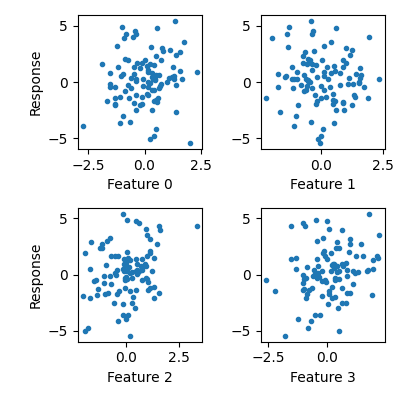
Visualize data

Some features are informative and others are not.

fig, axes = plt.subplots(2, 2)
for ii, ax in enumerate(axes.ravel()):
    ax.scatter(X[:, ii], y.ravel(), marker='.')
    ax.set_xlabel('Feature {}'.format(ii))
for ax in axes[:, 0]:
    ax.set_ylabel('Response')
fig.tight_layout()

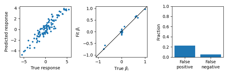
Fit a UoI-Lasso model

UoI-Lasso can fit low bias model parameters with feature selectivity. We can evaluate the predictions of the model, compare the fit \(\beta\), and look at the fraction of false positive and false negatives.

uoi_lasso = UoI_Lasso()
uoi_lasso.fit(X, y)
yhat = uoi_lasso.predict(X)

fig, axes = plt.subplots(1, 3, figsize=(7.5, 2.5))
ax = axes[0]
ax.scatter(y, yhat, marker='.')
ax.set_xlabel('True response')
ax.set_ylabel('Predicted response')

ax = axes[1]
val = max(abs(beta).max(), abs(uoi_lasso.coef_).max()) * 1.1
ax.scatter(beta.ravel(), uoi_lasso.coef_.ravel(), marker='.')
ax.set_xlabel(r'True $\beta_i$')
ax.set_ylabel(r'Fit $\beta_i$')
ax.set_xlim(-val, val)
ax.set_ylim(-val, val)
ax.plot([-val, val], [-val, val], c='k', lw=1.)

ax = axes[2]
fp = np.logical_and(uoi_lasso.coef_ != 0, beta == 0).mean()
fn = np.logical_and(uoi_lasso.coef_ == 0, beta != 0).mean()
ax.bar([0, 1], [fp, fn], align='center')
ax.set_xticks([0, 1])
ax.set_xticklabels(['False\npositive', 'False\nnegative'])
ax.set_ylabel('Fraction')
ax.set_ylim(0, 1)
fig.tight_layout()

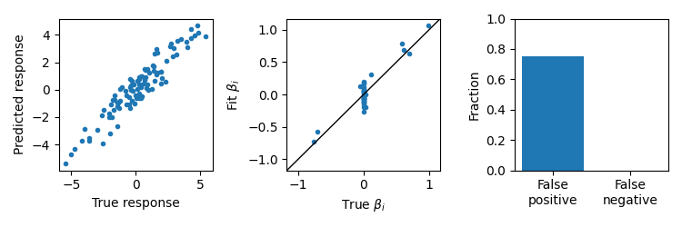
Ordinary Least Squares

OLS will have low bias fits, but will not generally have feature selectivity resulting in many false positives.

lr = LinearRegression()
lr.fit(X, y)
yhat = lr.predict(X)

fig, axes = plt.subplots(1, 3, figsize=(7.5, 2.5))
ax = axes[0]
ax.scatter(y, yhat, marker='.')
ax.set_xlabel('True response')
ax.set_ylabel('Predicted response')

ax = axes[1]
val = max(abs(beta).max(), abs(lr.coef_).max()) * 1.1
ax.scatter(beta.ravel(), lr.coef_.ravel(), marker='.')
ax.set_xlabel(r'True $\beta_i$')
ax.set_ylabel(r'Fit $\beta_i$')
ax.set_xlim(-val, val)
ax.set_ylim(-val, val)
ax.plot([-val, val], [-val, val], c='k', lw=1.)

ax = axes[2]
fp = np.logical_and(lr.coef_ != 0, beta == 0).mean()
fn = np.logical_and(lr.coef_ == 0, beta != 0).mean()
ax.bar([0, 1], [fp, fn], align='center')
ax.set_xticks([0, 1])
ax.set_xticklabels(['False\npositive', 'False\nnegative'])
ax.set_ylabel('Fraction')
ax.set_ylim(0, 1)
fig.tight_layout()

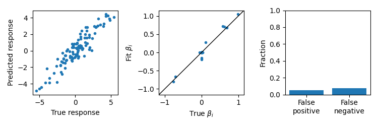
Cross-validated Lasso

Lasso can fit models with feature selectivity, but will have biased estimates of the parameters and will typically have more false positives and false negatives than UoI-Lasso.

lr = LassoCV(cv=5)
lr.fit(X, y)
yhat = lr.predict(X)

fig, axes = plt.subplots(1, 3, figsize=(7.5, 2.5))
ax = axes[0]
ax.scatter(y, yhat, marker='.')
ax.set_xlabel('True response')
ax.set_ylabel('Predicted response')

ax = axes[1]
val = max(abs(beta).max(), abs(lr.coef_).max()) * 1.1
ax.scatter(beta.ravel(), lr.coef_.ravel(), marker='.')
ax.set_xlabel(r'True $\beta_i$')
ax.set_ylabel(r'Fit $\beta_i$')
ax.set_xlim(-val, val)
ax.set_ylim(-val, val)
ax.plot([-val, val], [-val, val], c='k', lw=1.)

ax = axes[2]
fp = np.logical_and(lr.coef_ != 0, beta == 0).mean()
fn = np.logical_and(lr.coef_ == 0, beta != 0).mean()
ax.bar([0, 1], [fp, fn], align='center')
ax.set_xticks([0, 1])
ax.set_xticklabels(['False\npositive', 'False\nnegative'])
ax.set_ylabel('Fraction')
ax.set_ylim(0, 1)
fig.tight_layout()
plt.show()